
Mainframes and Supercomputers, From the Beginning Till Today.
This article is provided by guest author max1024, hailing from Belarus. I have provided some minor edits/tweaks in the translation from Belarusian to English.
Mainframes and Supercomputers, From the Beginning Till Today.
Introduction
We all have computers that we like to use, but there are also more productive options in the form of servers with two or even four processor sockets. And then one day I was interested, but what is even faster? And the answer to my question led me to a separate class of computers: super-computers and mainframes. How this class of computer equipment developed, as it was in the past and what it has achieved now, with what figures of performance it operated and whether it is possible to use such machines at home, I will try to explain all this in this article.
FLOPS’s
 First you need to determine what the super-computer differs from the mainframe and which is faster. Supercomputers are called the fastest computers. Their main difference from mainframes is that all the computing resources of such a computer are aimed at solving one global problem in the shortest possible time. Mainframes on the contrary solve at once a lot of different tasks. Supercomputers are at the very top of any computer charts and as a result faster than mainframes.
The need for mankind to quickly solve various problems has always existed, but the impetus for the emergence of superfast machines was the arms race of well-known superpower countries and the need for  nuclear calculations for the design and modeling of nuclear explosions and weapons. To create an atomic weapon, colossal computational power was required, since neither physicists nor mathematicians were able to calculate and make long-term forecasts using the colossal amounts of data by hand. For such purposes, a computer “brain” was required. Further, the military purposes smoothly passed into biological, chemical, astronomical, meteorological and others. All this made it necessary to invent not just a personal computer, but something more, so the first mainframes and supercomputers appeared.
 The beginning of the production of ultrafast machines falls on the mid-1960s. An important criterion for any machine was its performance. And here on each user speaks of the well-known abbreviation “FLOPS”. Most of those who overclock or test processors for stability are likely to use the utility “LinX”, which gives the final result of performance in Gigaflops. “FLOPS” means FLoating-point Operations Per Second, is a non-system specific unit used to measure the performance of any computer and shows how many floating-point arithmetic operations per second the given computing system performs.
 “LinX” is a benchmark of “Intel Linpack” with a convenient graphical environment and is designed to simplify performance checks and stability of the system using the Intel Linpack (Math Kernel Library) test. In turn, Linpack is the most popular software product for evaluating the performance of supercomputers and mainframes included in the TOP500 supercomputer ranking, which is made twice a year by specialists in the United States from the Lawrence Berkeley National Laboratory and the University of Tennessee.
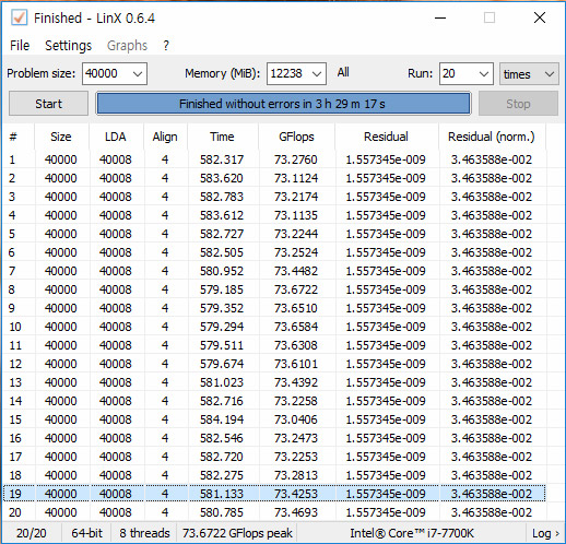
When correlating the results in Giga, Mega and Terra-FLOPS, it should be remembered that the performance results of supercomputers always are based on 64-bit processing, while in everyday life the processors or graphics cards producers can indicate performance on 32-bit data, thereby the result may seem to be doubled.
The Beginning
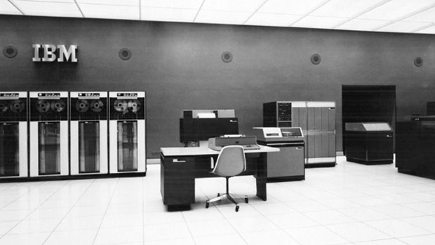
IBM S/360
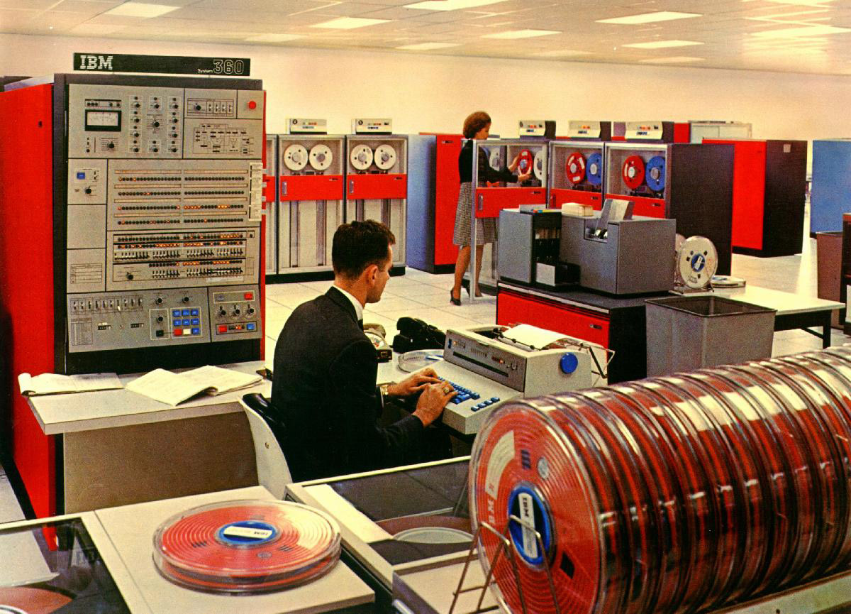
The first mainframe was created by the well-known IBM in 1964, while the cost of its creation amounted to $5 billion. To adjust for inflation to 2018 dollar this figure should be multiplied by 6-7. This supercomputer was called IBM System/360 (S/360), it was not enclosed in the usual monolithic case, but consisted of various modules and weighed more than one ton (2000lbs/900kg) . In total IBM announced 6 models of this system and 40 various peripherals.
The performance of such a mainframe, depending on the model, was from several thousand operations per second, to a million. At the heart of the system were integrated circuits, which totaled from tens to hundreds of thousands of transistors. The amount of RAM, depending on the model, was from 16 to 1024 Kb, although in a super maximum configuration, the volume could be as much 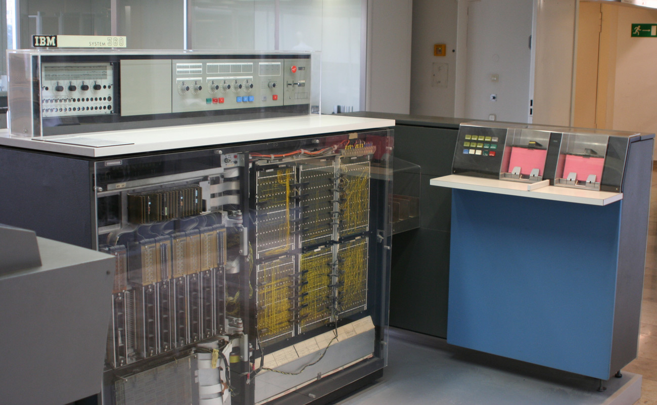 as 16 MB. All the processed information was stored on giant reels with a magnetic tape, which had 9 tracks. Hard drives were also released, the volume of which was couple megabyte, and the weight of a couple tens of kilograms. There was also an option for storing information on memory with magnetic cores of a couple of megabytes in size.
By today’s standards, the figures are microscopic, but from them all began. With the announcement of the IBM System / 360, such modern standards were introduced, which still remain. So for the first time one byte was equal to eight bits, byte memory addressing, 32-bit words were introduced. In older models, the technology of dynamic address translation (dynamic address translation), which is known to us as “virtual memory”, has been implemented.
IBM S/360 with peripherals
Cray-1 – 1976
Despite its high cost (up to 3 million dollars), IBM System / 360 sales were going with a Hooray! During the first month of IBM, orders were received for more than a thousand copies of such machines, and in the 6 years of the family’s existence, more than 33,000 such machines were sold. Thus IBM System / 360 mainframe laid the foundation and further development trends of computer equipment.
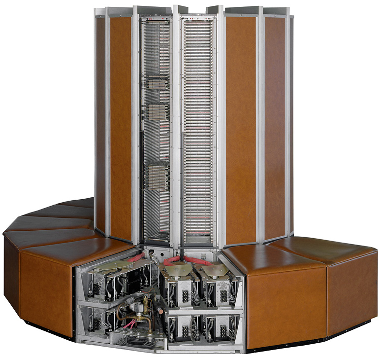
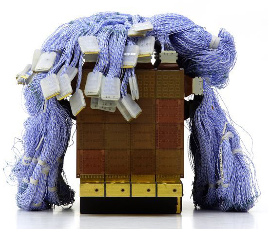
Cray-1 was a vector-pipeline computing system, the central processor consisted of 500 circuit boards, on which there were 144,000 chips, which in turn operated at a frequency of 80 MHz. The chip supplier was Fairchild, from which the founders of Intel and AMD subsequently came out. The amount of RAM was 8 megabytes. All boards were installed in a tower shell with 12 sections, when viewed from above the form of the supercomputer resembled the outline of the letter “C”.
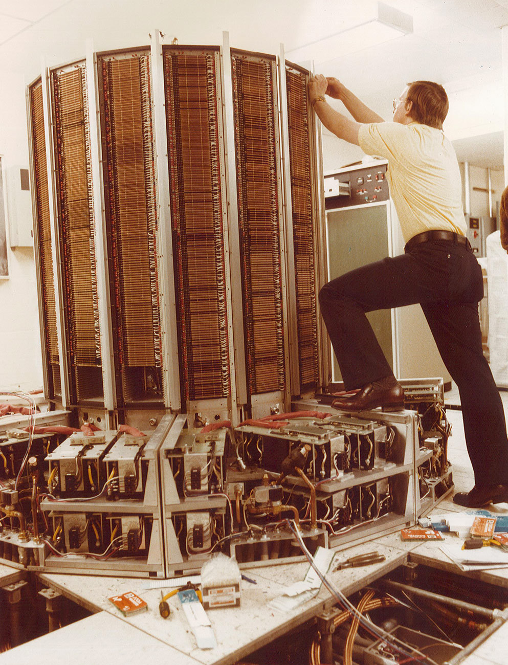
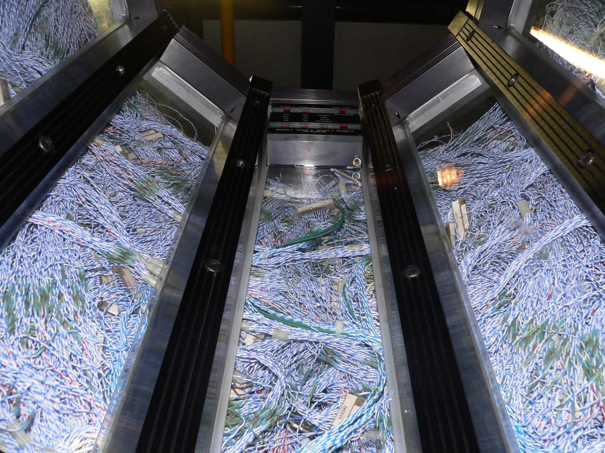 To improve performance and reduce delays during the passage of signals, Seymour Cray invented and designed a special form factor for his machine, the main idea was to reduce the distances between boards, so the shape of the main skeleton was chosen in the form of a polyhedron, which made it possible to surround the perimeter of the processor with memory chips, in As a result, the access time to each of them was the same. Also, this arrangement of the boards made it possible to shorten the length of the wires and provide a better heat dissipation. But despite these optimizations, the number of wires inside the Cray-1 is amazing.
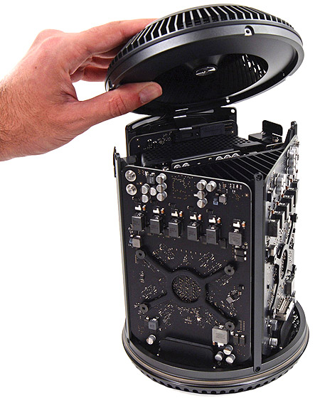
The tower design of the Cray-1 reminded me of the cylindrical Apple Mac Pro, only in a much reduced form.
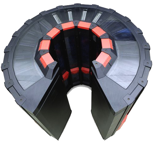
Cray-1 Cooling
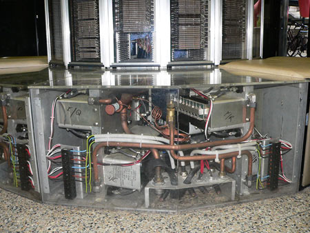
The performance of the system exceeded 100 MFLOPS, and in tasks optimized for the vector processor, it reached 150 MFLOPS. The weight of the Cray-1 was 5.25 tons (4760kg), a height of about two meters, the total power consumption was 250 kW, 135 of which were used in the compressor cooling system operating with liquid Freon. The logic IC’s of the Cray-1 were all ECL (Emitter Coupled Logic) which is very fast but generated a lot of heat. Liquid Freon circulated through 12 steel main pipes inside the system housing, taking heat from the circuit boards with microcircuits, to which copper plates with Teflon coating adhered for more efficient heat removal. At the bottom of the Cray-1 was the refrigeration unit.
Here is an example of Cray-1 boards, which are now being sold at the worldwide Ebay auction as relics. When one IC failed, the whole board was changed, the repair of the failed component on the board was not envisaged.
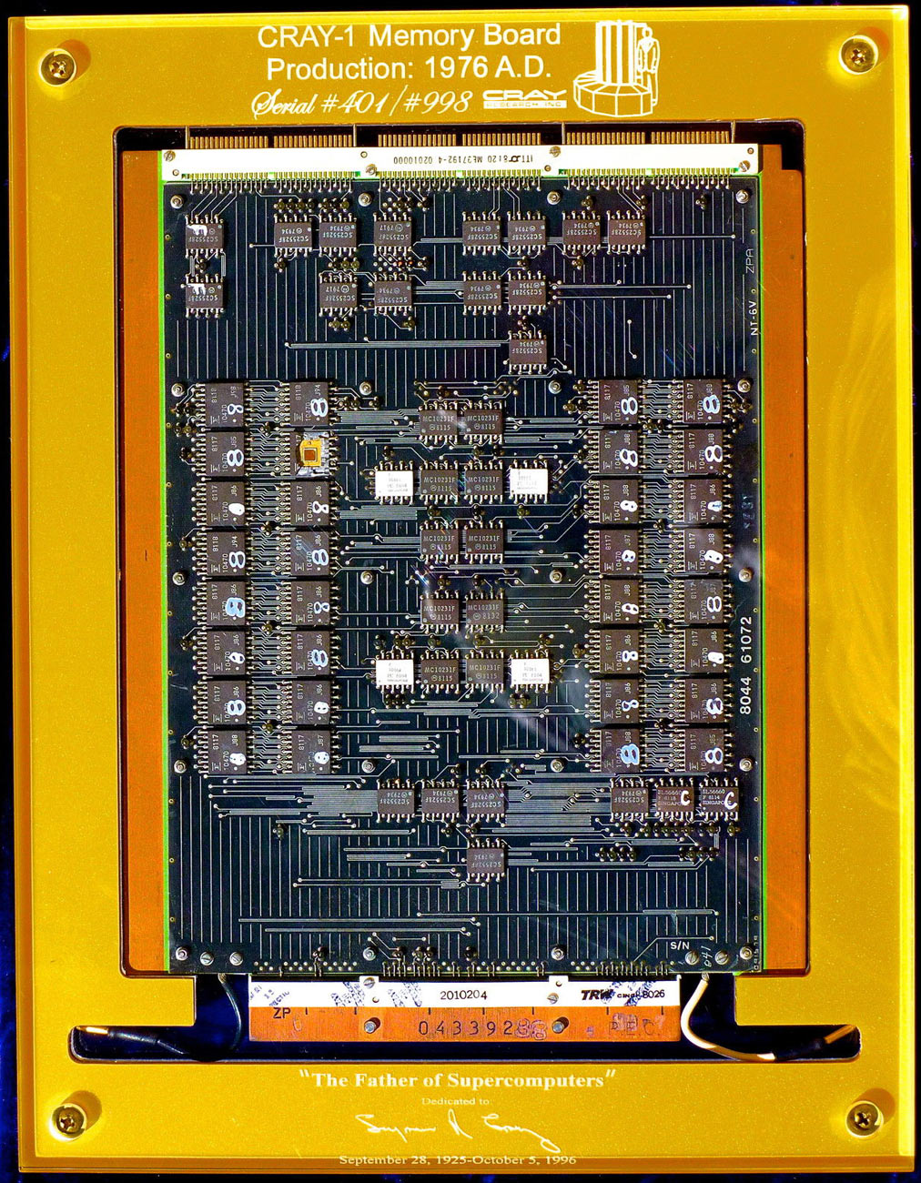
Cray-1 Bipolar Memory Board
The peculiarity of the Cray-1 architecture was that it had the ability to adapt to the structure of the problem 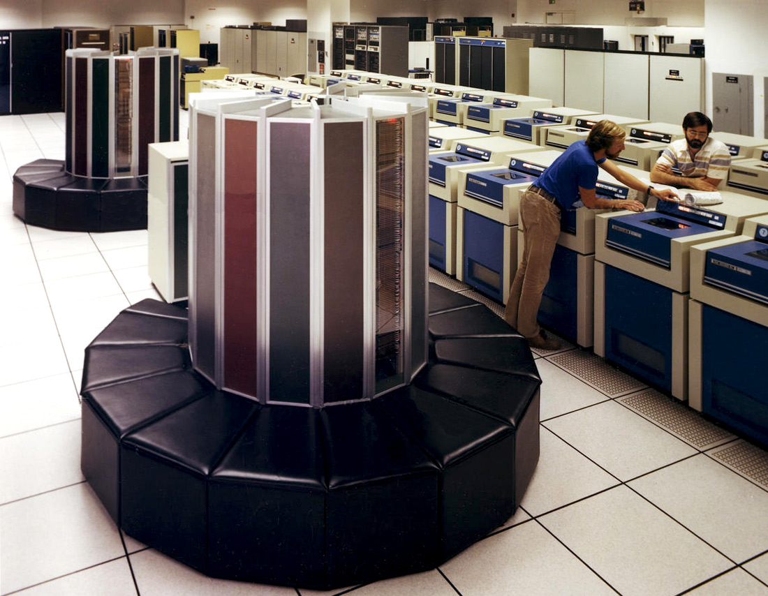 being solved, parallel operation of both pipelines and elementary processing units within any pipeline was allowed. The system was able to perform both scalar and vector operations, and simultaneously several scalar and vector operations could be performed. The operating system was COS (Cray Operating System), which provided a batch processing mode for up to 63 tasks.
For customers of this supercomputer was available a kind of modding, the customer could choose the color of  the faces at his discretion. For those who did not have enough money to buy, it was planned by Cray to be able to rent a supermachine. The monthly subscription cost was $210,500. Since the release of the first supercomputer to the end of its production, Seymour Cray had sold 85 Cray-1 systems, becoming the world leader in the production of the most productive computing systems in the World.
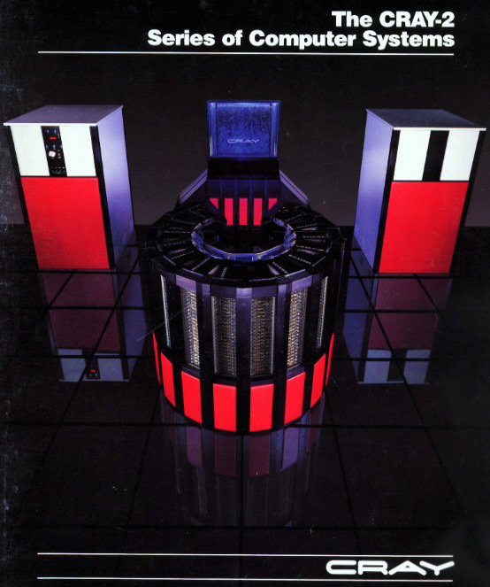
In the spring of 1985, Seymour Cray introduced his new and fastest computer, the Cray-2, built to the order of the US Department of Defense, which claimed supremacy among all the supermachines before 1990. This supercomputer was significantly different from its predecessor. For 10 years the productivity has grown many times and reached 1.9 GFLOPS. The amount of RAM was 2 GB. The number of processors was increased to 4 ‘cores’ and to each of them, in addition to vector registers, a local RAM of 128 KB was added. The clock frequency of each processor was 244 MHz, and the processing power was 488 MFLOPS.
Cray 2
Appearance was in the form of the same cylinder, but its dimensions and weight decreased. The height of the
Cray 2 Brochure
cabinet was 1.15 meters, and weight ~2500 kg. Power consumption was down to around 195 kW. The cost of one machine was set at around $ 17.5 million, by today’s dollars it’s about $ 36 million.
Due to the reduced size and denser layout of the boards, the Freon cooling system was no longer suitable. Seymour Cray once again proposed an innovative approach in the form of using a liquid cooling system. Inside the hermetically sealed Cray-2, a special inert coolant was flooded, developed by 3M, which took all the heat, generated by the supercomputer. The volume of coolant was about 760 liters (200 gallons), which was about 1/3 of the mass of the device. When the elements were heated on the transparent walls of the Cray-2, numerous bubbles appeared. With modern RGB backlighting, this supercomputer would look much better =) But this fluid had one negative property, when it boiled, gasses that were rather dangerous for human health were created, therefore, the case was hermetically sealed.
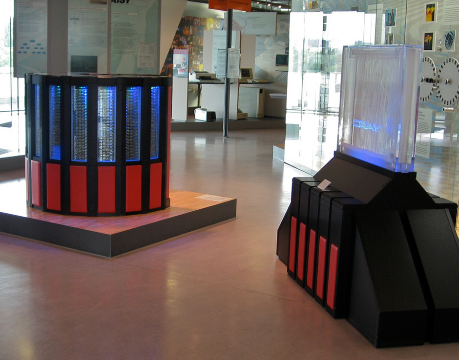
Cray 2 with Fluorinert-cooling “waterfall”on the right
The Cray-2 was able to connect to another Cray-2 to increase processing power.
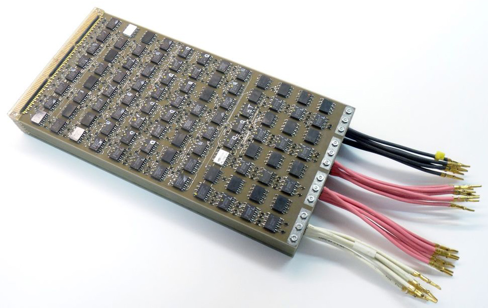
Cray 2 ECL Logic Board
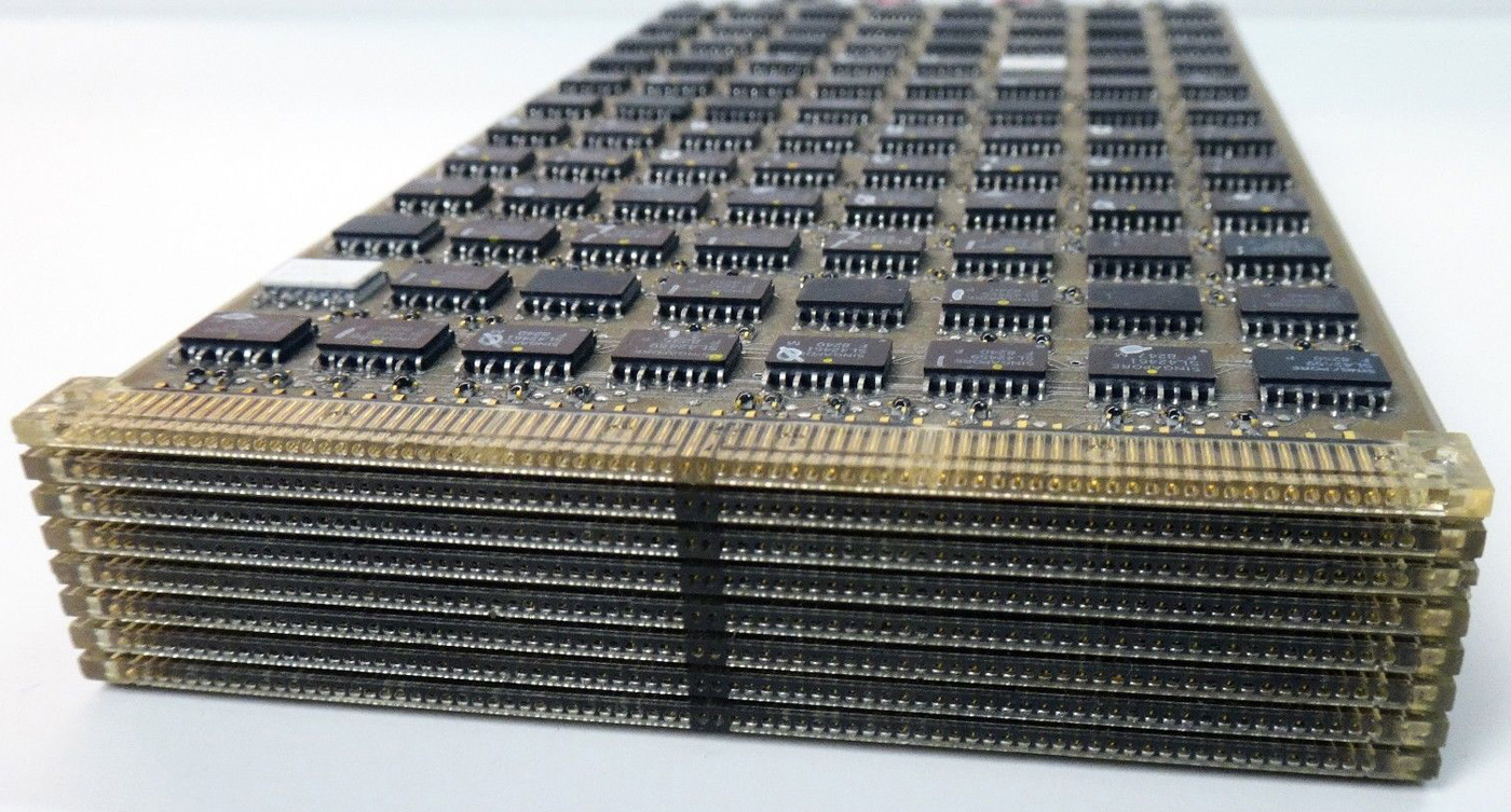
Cray 2 Logic Module
The connection was made through a dedicated network with a capacity of 1.6 Gbit/s. Since the mid-80s, the role of software has begun to increase, and the costs of its design have grown significantly. So the development of software for Cray-2 was the same amount of as on its hardware. The operating system for the Cray-2 was a UNIX operating system, something that has become rather standard in supercomputers to this day (UNIX/LINUX in many flavors).
In the following year, in 1990, an 8-processor Cray-2 costing $ 19 million was built exclusively for the
Cray 3 Wiring
Livermore National Laboratory, which is now in the Museum of Computer History in California, USA. After that, all efforts were made to develop the next model of the supercomputer – Cray-3, but due to a number of problems in the development, only one copy of Cray-3 was built. Its computing power was 5 GFLOPS.
Interestingly, the Cray-3 was modeled on Apple’s computers, and Apple in its turn bought a Cray supercomputer to assist with the design of its PCs. Cray supercomputers were used not only for military purposes, their power was used in NASA, but also to create special effects in the film industry, which was already beginning to move away from using models and began using all the power of supercomputers to create special effects. The Cray-2 capacities were used in such blockbusters as “Star Wars”, “Jurassic Park”, “Terminator 2: Judgment Day”, etc.
Fujitsu Numerical Wond Tunnel
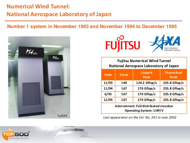
If from the very beginning of the market of supercomputers dominated Americans companies, then from the beginning of the 90s of the last century Japanese manufacturers began to join the competition. One such manufacturer was Fujitsu, which in 1993 created its vector parallel supercomputer called the Numerical Wind Tunnel in cooperation with the Japan National Aerospace Laboratory. In the Linpack test, it showed a performance of 124.2 GFLOPS. It was based on 140 vector processors with a clock frequency of 105 MHz produced by Fujitsu itself using GaAs technology (Gallium Arsenide, vs Silicon). In the following year, their number was increased to 166 processors. The total RAM was 44.5 GB or 256 MB per node. The total system power consumption was 498 kW. The cooling system was two-cascaded, first cooled chips with microcircuits, and the second – brought heat outside the building.
In March 1996, the Japanese company Hitachi also released its supercomputer with the uncomplicated name SR2201/1024. In this system 1024 scalar HARP-1E processors based on the PA-RISC 1.1 architecture with a clock speed of 150 MHz were used, which were able to develop the performance in 220.4 GFLOPS. These processors were manufactured by Hewlett-Packard who had originally developed the PA-RISC architecture.
Hitachi SR2201/1024
Each of the 1024 nodes had 256 MB of RAM at its disposal, which totaled 256 GB and was connected to other nodes via a high-speed interface capable of providing data transfer at the level of 300 MB/s. The amount of disk space was 72 GB. This supercomputer was located at the Tokyo University in Japan.
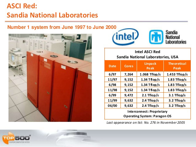
The first supercomputer that broke 1000 GFLOPS or 1 teraflops was the Intel ASCI Red, built in 1997.

IBM ASCI Red
It was based on, 9152 regular, freely available at that time, Intel Pentium Pro processors with a clock speed of 200MHz using Socket 8. Each node contained two such processors and 128 MB of RAM.
A couple of such nodes were located on a common board with a communication module, which were housed in 85 rack cabinets. The total amount of RAM in Intel ASCI Red was 594 gigabytes; the disk subsystem consisted of 640 HDDs with a total disk space of 2 terabytes.
This “teraflop” supercomputer was built by Intel itself, commissioned by the US government at a cost of around $ 55 million. The main architectural criterion was the use of commodity components, so the commercial server components of that time were chosen, but with the exception of the communication modules that were
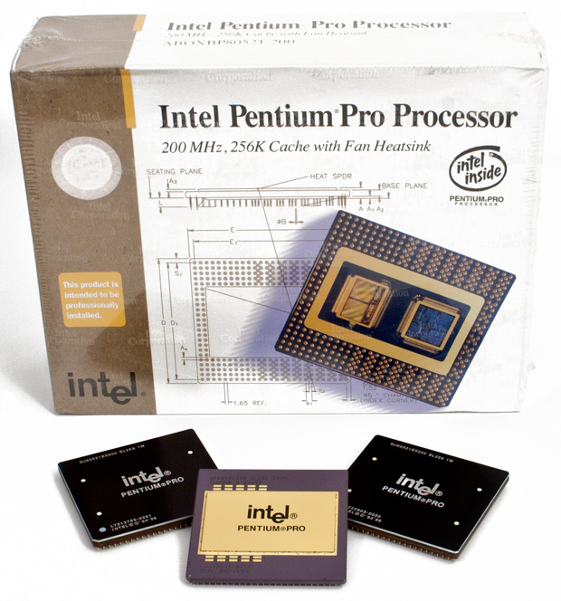
Intel Pentium Pro Processors
specifically designed for ASCI Red. The main purpose of the machine was to monitor the US nuclear arsenal after the announcement in October 1992 of a moratorium on nuclear testing.
All equipment was located in an area of 150 square meters (1600 sqft.) and consumed 850 kW of energy and another 500 kilowatts was required for air conditioning the room to maintain the optimum operating temperature of the supercomputer. In the Linpack test, the supercomputer showed the result of 1.338 TFLOPS.
In 1999, the Intel ASCI Red upgrade was ripe and Intel again took the lead. Thanks to this event, a unique processor using the Socket 8 but with the power of the Pentium II – the Pentium II OverDrive operating at 333 MHz appeared. The “charged” Intel ASCI Red version 2.0 with 9632 processors after the upgrade showed performance at 2.38 TFLOPS in the Linpack test.
ASCI Red Upgrade Timeline
These quality characteristics allowed Intel ASCI Red to retain the title of the fastest supercomputer from June 1997 to June 2000.
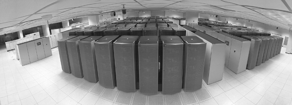
Processor capacity is never small, and therefore, under the order of the US government, within the framework of the development of supercomputer technologies, within the third phase of the Advanced Simulation and Computing Program (ASCI) program, a tender was announced to build an even more powerful supercomputer. Each stage of the ASCI program assumed an increase in the power of the new supercomputer compared to the previous one by about 2.5 times. This time, IBM was awarded the honor of being the creator of the new teraflops conqueror. In February 1998, it was officially announced that IBM received a contract for the construction of a new supercomputer, which would be called ASCI White, and on August 15, 2001 it was officially handed over to the customer and installed at the Livermore National Laboratory.
ASCI White
What was ASCI White, which cost $ 110 million? This is a cluster of SMP-servers consisting of 512 machines connected by its new communication technology “Colony” with a bandwidth of about 500 MB/s. The total number of IBM POWER3 processors with a clock speed of 375 MHz was 8192 cores.
IBM POWER3-II 375MHz
At the disposal of the supercomputer were 6 TB of RAM and 160 TB of disk space. The size of ASCI White was comparable to the area of two basketball courts, and the weight of all equipment was 106 tons.
ASCI White Cabinetry
The total length of the cables for connecting all the components was 64.3 kilometers (40 miles). To lay all the kilometers of cables had to raise the floor to a height of 60 cm allow for room for routing cables.
ASCI White: Raised floor was needed to allow routing of all the wiring.
The power consumption of ASCI White was 3 Megawatt of electricity and the same amount was required for cooling. All this power showed the result in the LINPACK test in 7.3 TFLOPS.
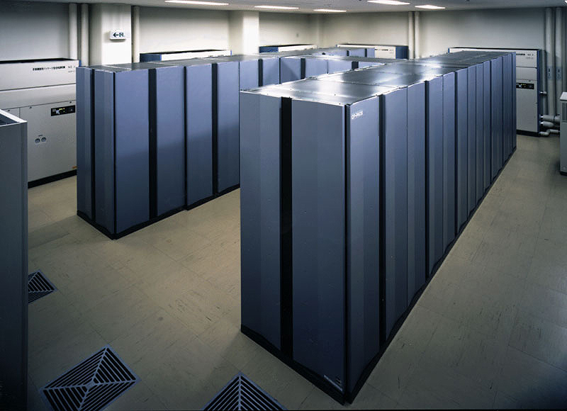
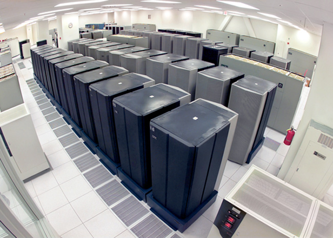
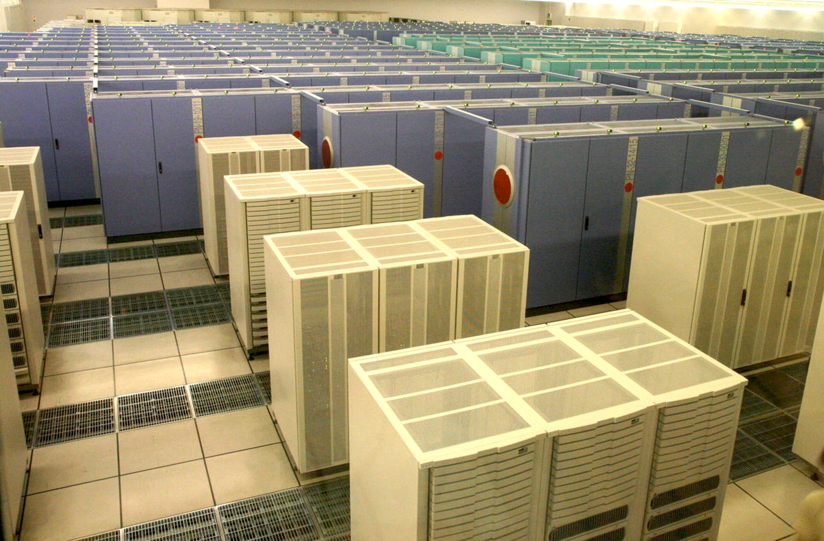
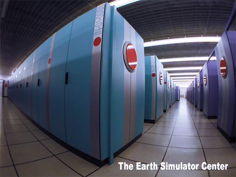
In 2002, the leader’s jersey again moved to the country of the rising sun. By order of the Japanese government, the Japanese company NEC built a supercomputer with a real capacity of 35.86 TFLOPS. A Japanese computer called Earth Simulator, it was developed specifically for the Japanese Science and Technology Agency for climate, tectonic, atmospheric and other calculations. In fact, a small model of our planet was constructed to predict various natural phenomena and disasters.
NEC Earth Simulator
NEC Earth Simulator was 5 times faster than IBM ASCI White and 3.5 times more expensive. Around 350 million US dollars was spent on its development. For its installation a two-story pavilion of 65 meters in length and 50 in width was built. 640 nodes with 8 vector processors and 16 gigabytes of RAM in each node combined 5120 processors and 10 terabytes of RAM in total. The processor frequency was 500 MHz, but some of its components support operation at a frequency of 1 GHz.
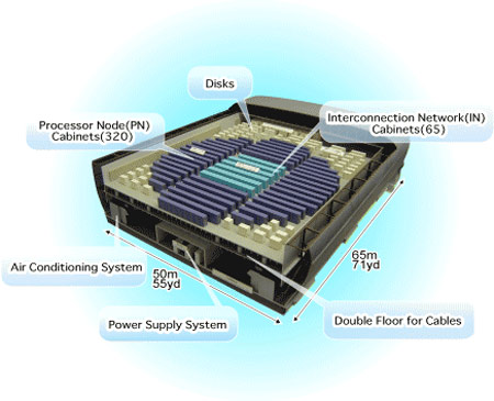
NEC Earth Simulator System Layout
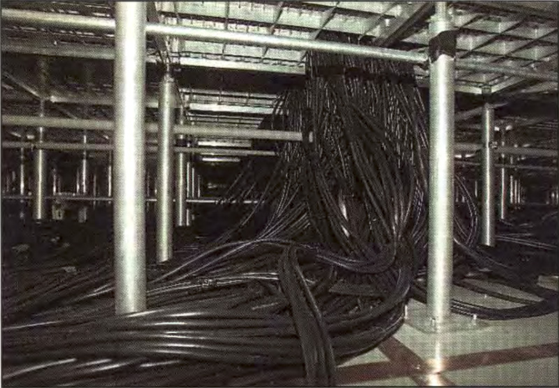
The system of hard disk storage consisted of a HDD with a total volume of 700 TB, plus a tape library named StorageTek 9310 with a volume of 1.6 Petabytes. The amount of energy consumed was 6.4 megawatts, and this without the cost of cooling, so a small substation of 20 MW was built nearby.
Earth Simulator
To connect all components, 83,200 cables with a total length of 2400 km (~1500 miles) were required. The bidirectional data transfer rate for each channel connecting the processor nodes to the switch was 12.3 GB/s. In 2009 and further in 2015, NEC released the second and third generation of “Earth Simulator”. By the way, the last generation of Earth Simulator (ES3 – 2015) shows a performance of around 1300 TFLOPS.
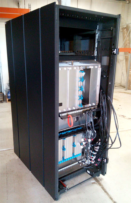
IBM Roadrunner
The first supercomputer that broke the threshold for a petaflops for the first time was – IBM Roadrunner, built naturally by IBM itself and installed by the Los Alamos National Laboratory (USA) for nuclear weapons
IBM PowerXCell 8i
research in 2008. In addition, it was the first hybrid supercomputer that uses simultaneously two essentially different processor architectures. So, IBM Roadrunner consisted and worked harmoniously with each other: 6480 dual-core AMD Opteron 2210 processors with 1.9 GHz frequency and 12,960 IBM PowerXCell 8i processors running at 3.2 GHz frequency (similar to those used in Sony Playstation 3).
This supercomputer, like the Intel ASCI Red, is made from commercial components, it includes IBM Model QS22 blade servers, which are housed in 278 cabinets. For communication, 10,000 Infiniband connections and about 90 km (56 miles) of fiber optic cable were used. The total amount of RAM of this monster was 98 terabytes, weight – 226 tons, consumed power: 3.9 megawatts, for development it took more than 120 million US dollars.
Standard processing (for example, file system I/O) is handled by AMD Opteron processors, mathematical and processor calculations are handled by the Cell processors. IBM Roadrunner has been working with open source Linux software from Red Hat.
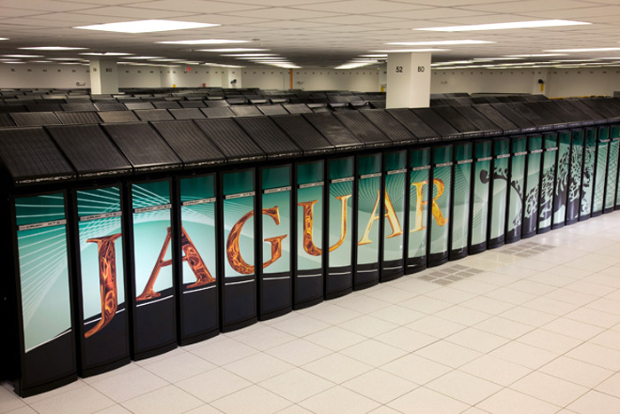
Cray XT5 Jaguar
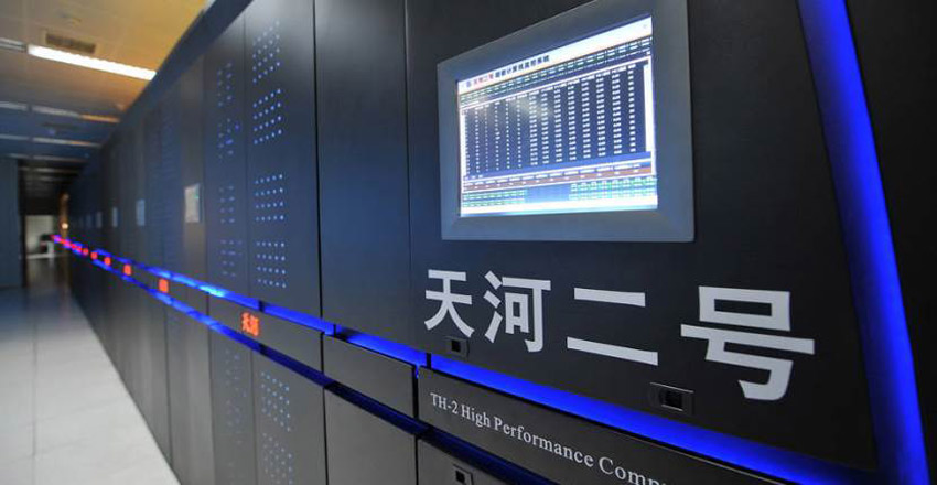
Further from 2008, the race for the conquest of petaflops began. At the end of 2009, the supercomputer Cray XT5, also known as the “Jaguar,” in the Linpack test shows a performance of 1.759 PFLOPS. In 2010, the supercomputer from the People’s Republic of China, Tianhe-1A shows a performance of 2.57 PFLOPS. In 2011, the Japanese supercomputer – K Computer demonstrates the result in 8.16 quadrillion operations per second. But the supercomputer named Titan and again built by Cray is more interesting.
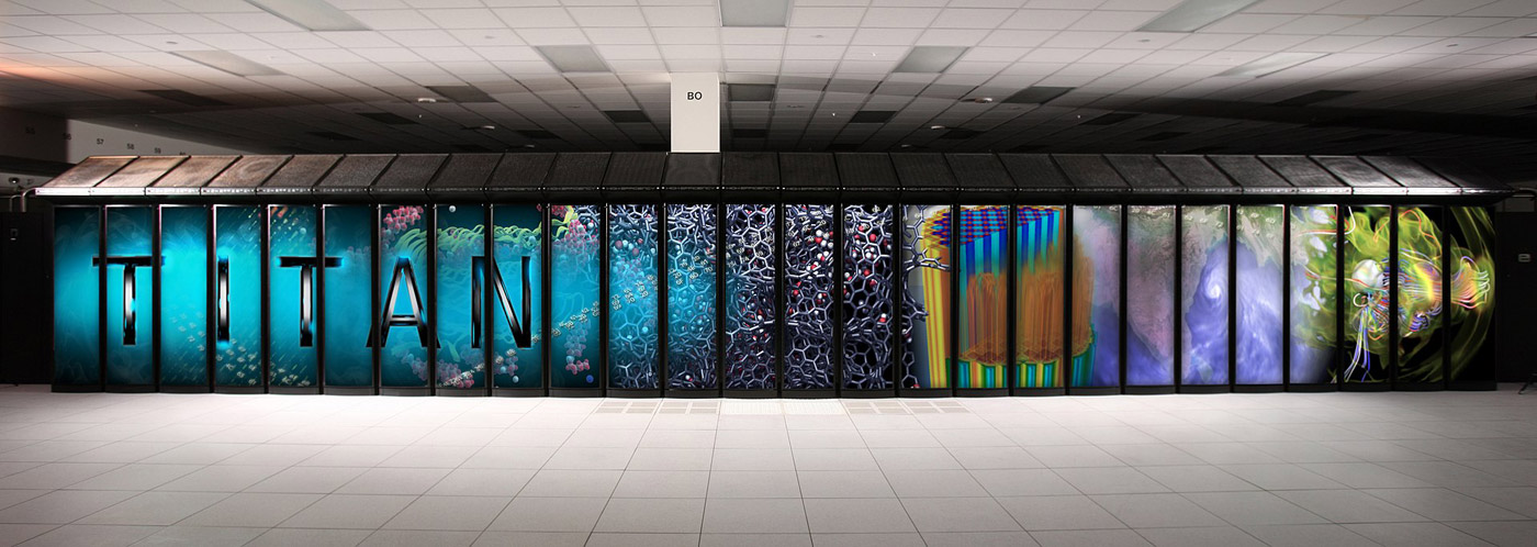
Cray XK7 Titan
Essentially, the Titan supercomputer, aka the Cray XK7, was an upgrade to Jaguar, which operated at the US
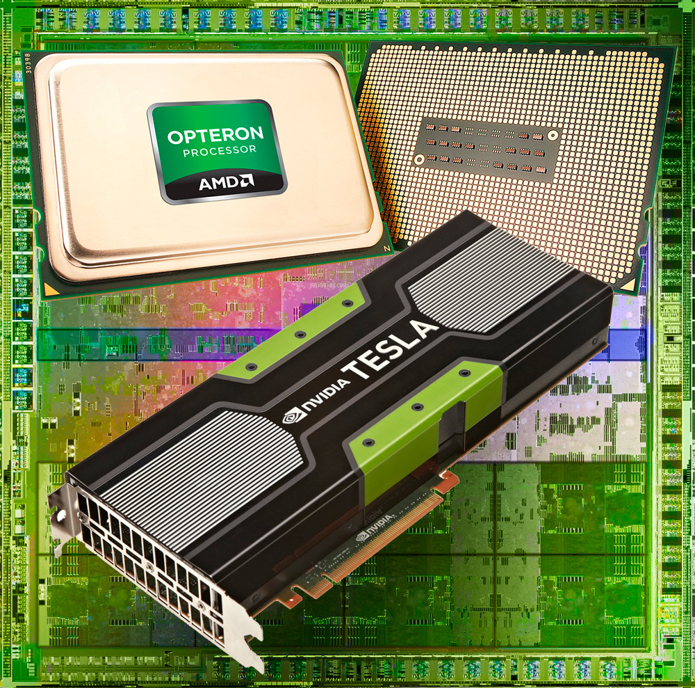
AMD Bulldozer and Nvidia Kepler
Department of Energy’s National Laboratory. The $ 60 million upgrade included 18688 sixteen core AMD Opteron 6274 (Socket G34, Bulldozer microarchitecture, the price at the announcement of $ 639) operating at 2.2 GHz frequency and 18,688 server GPUs Nvidia Tesla K20X (microarchitecture Kepler, the cost at the time of the announcement of $ 3199, similar to the NVIDIA GTX TITAN first generation). The power of one Nvidia Tesla K20X with six gigabytes of memory onboard is 1.31 TFLOPS.
Such a heterogeneous neighborhood of components allowed Titan to demonstrate impressive performance at 17.6 PFLOPS. The total amount of Titan’s RAM was 710 TB, the amount of disk subsystem was 40 Petabytes, and the power consumption was 8.2 MWatt.
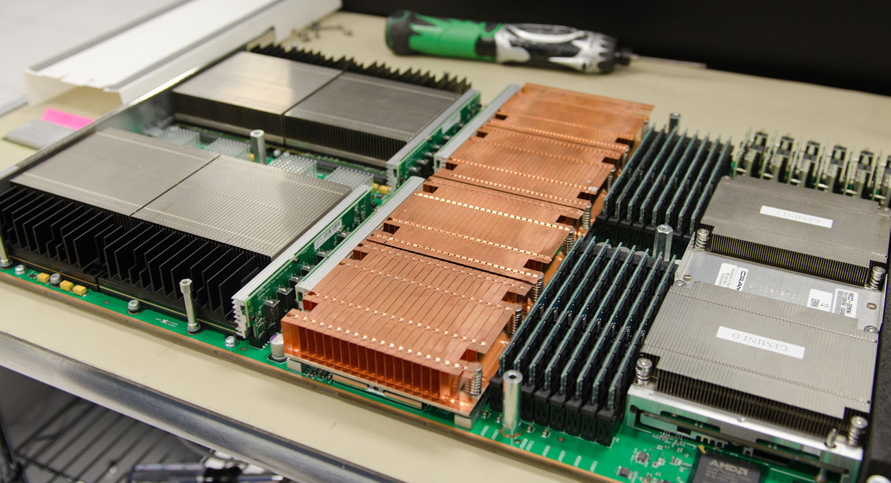
Titan PCB
Nowadays, the Titan from Cray, despite the passing of five and a half years from the moment of its launch to the present day, occupies the 5th line of the TOP-500 World Ranking. At this point in time (1H2018), the top five leaders are as follows:
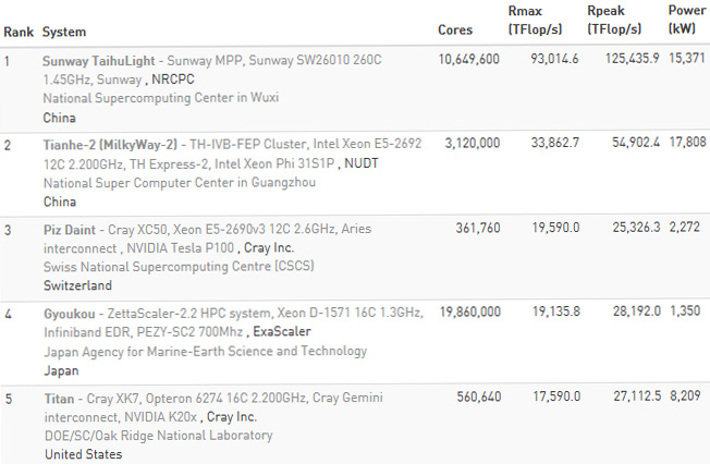
Top 500 Top 5 1H2018
The first line is occupied by a supercomputer with an astonishing amount of computing cores from called – Sunway TaihuLight, which in the Linpack test demonstrated the result of 93 PFLOPS! At the heart of this
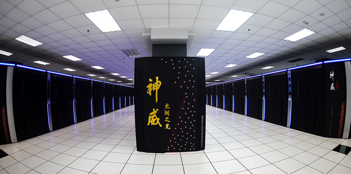
Sunway TaihuLight
supercomputer are a domestic Chinese development, that is, 260-core 64-bit RISC-processors of its own production with a clock frequency of 1.45 GHz. Sunway TaihuLight uses a total of 10 million processor cores, with each kernel capable of executing several instructions.
The amount of RAM is 1.31 Petabytes, the power consumption is 15 MWatt. The total amount of disk space is 20 petabytes. Structurally, the supercomputer consists of 40 water cooled racks with a peak performance of each rack in 3 PFLOPS.
The Sunway TaihuLight supercomputer is the development of specialists of the National Research Center for Parallel Computer Computing and Technologies and installed in the National Supercomputer Center in Wuxi. To develop this supercomputer, it was spent 273 million dollars.
Sunway TaihuLight
Now China is building a new high-performance next generation computer – Tianhe-3, which will be at least 10 times faster than Sunway TaihuLight. The future supercomputer must overcome a new performance boundary of 1 exaflops (1,000,000,000,000,000,000,000, one million trillion) floating point operations per second. Presumably the construction will end in 2020, it remains to wait for this moment.
Supercomputer Processors
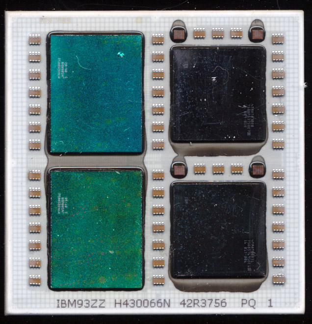
IBM Power5+ QCM
As you have already noticed, supercomputers used a variety of processors, from a set of countless chips on a printed circuit board, serially produced and freely found in the everyday retail of the model, to specially manufactured ones for building supercomputers. The latter are of the greatest interest. As a rule, such processors have several processor cores on one substrate and dies of which, if it is possible to remove the heatspreaders, glow with all the colors of the rainbow. I will give a few examples.
Above, you can see the IBM POWER5 + processor in QCM (Quad Chip Module) packaging. 8 cores of the processor work at 1.8 GHz frequency, next to them there are 72 MB of L3 cache memory. The Pentium Pro also has a similar packaging, a single processor core and a second level cache (L2) are on different dies.
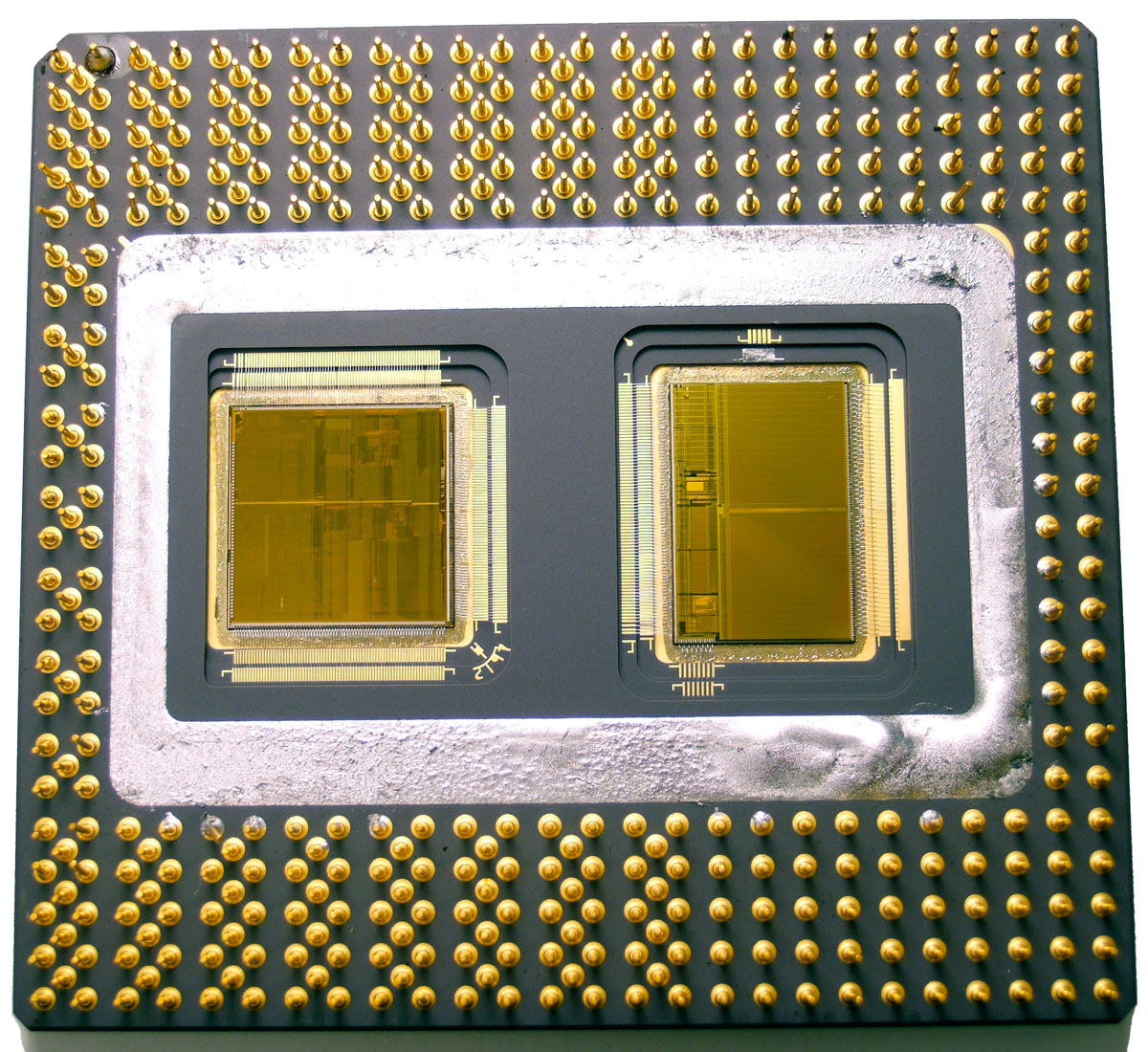
Pentium Pro – CPU die on left 256K Cache die on right
And this is how it looks, for example IBM Power4 CPU without a heat spreader:
IBM POWER4+
The case of the processor is made of strong ceramics and to remove the same ceramic cover is far from easy. You have to use brute force and a special tool. As progress progressed under the cover of such processors, the number of dies increased and the sizes of the processors grew, which acquired massive steel frames, and some models including fittings for the connection of water/oil cooling.
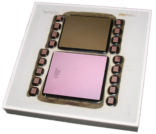
IBM z10 Processor MCM
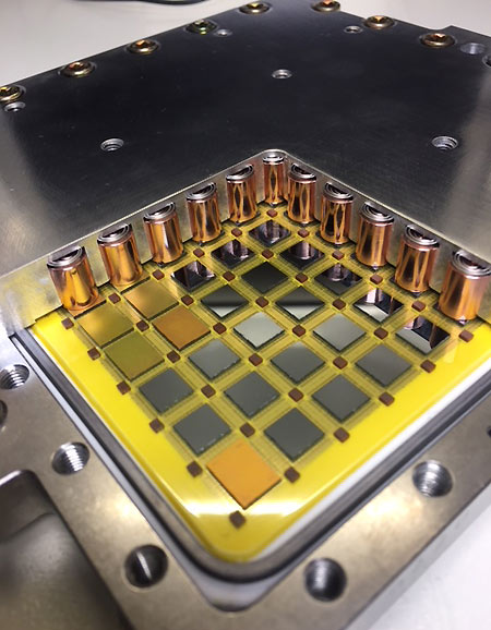
Above, you can see the IBM Z10 processor, specially released for mainframe in 2008. This “modular” processor has five quad-core processors with a frequency of 4.4 GHz, as well as two memory controllers. L2 cache memory is 3MB for each core and in addition to it, depending on the model, there may be another 40 to 48 MB of L3 cache. The size of this processor is truly impressive.
Below you can see one more “monster” – IBM Z196.
IBM z196
This processor is a multi-chip module and IBM has also been specially developed for its supermachines in 2010. The 512.3 mm2 chip consists of 1.4 billion transistors. Production technology is 45 nm, clock speeds up to 5.2 GHz. In addition to the 24 MB shared L3 cache, there are two dedicated companion chips called the Shared Cache on the processor module, each of which adds the L4 cache memory to 96 MB, which makes the total L4 cache total of 192 MB.
IBM MCM
Well, then the processors are just real giants:
IBM MCM Cutaway – ©cpu-galaxy.at
For installing such processors, such ready-made modules with a handle are used for their convenient installation.
MCM with installation handle
Disassembling such a processor module is not an easy task, sometimes you need to have a similar set of tools (below in the photo) and even a gas burner does not hurt, the method with the grip applicable for desktop CPUs will not work here. We will disassemble the example of IBM Power 4 in the pictures:
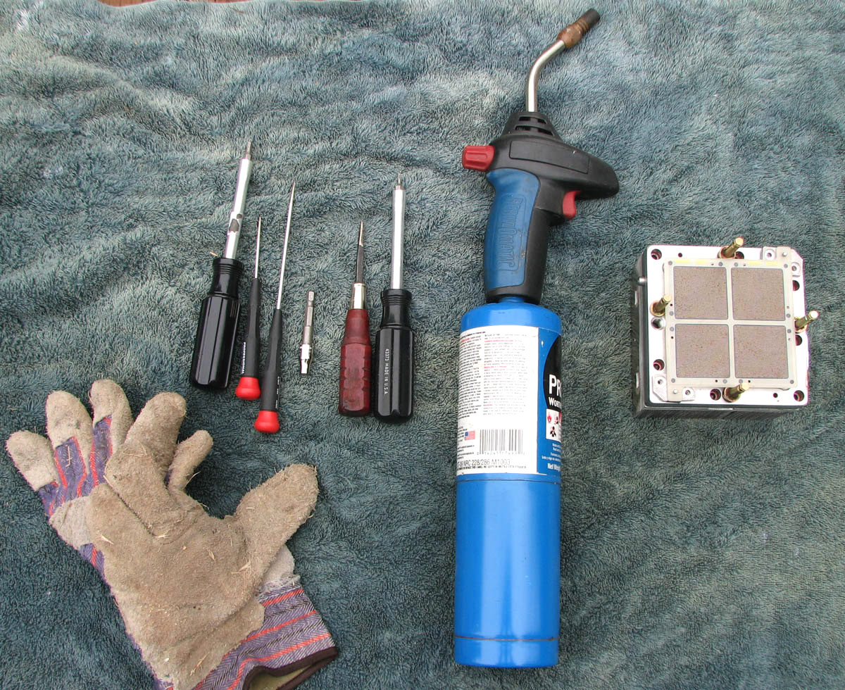
POWER4 Disassembly – Full article here
Mainframe at Home
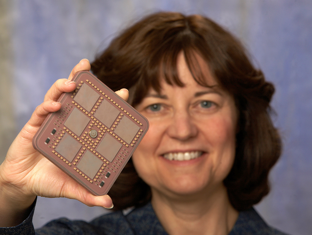
IBM z8901
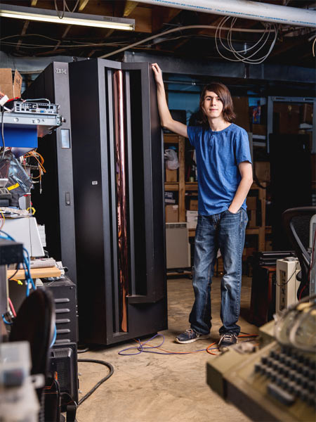
Is it possible to use a mainframe or a supercomputer at home? Why not. The main thing is desire, and the mainframe will be 😉 Perhaps not everyone knows, a couple of years ago in the internet flew the news that an 18-year-old college student in Maryland, Connor Krukosky, gathered in the basement of his home an IBM z890 mainframe which in 2004 was worth more than $300,000. He managed it thanks to participation in the auction on the site “GovDeals”, where one of the universities got rid of the old hardware. In addition to the only one bid by Connor Krukovski was $237, no one else bid and so he purchased a used mainframe for the grand sum of $237
The weight and dimensions of the IBM z890 are not small, it’s not a personal computer. With dimensions of 79 x 158 x 195 cm and a weight of 680 kg, this computing device is not easily transported and placed indoors. But there is nothing impossible.
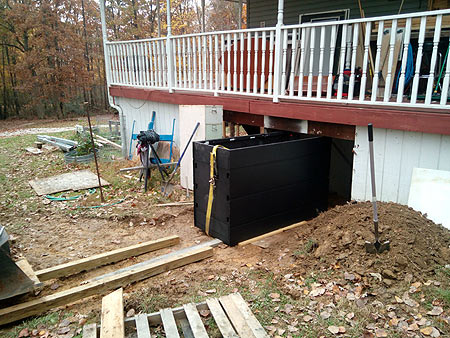
Into the basement…
After the operation to transport it to the basement, the mainframe was assembled and connected.
$237 IBM z8902 up and running
As a result, thanks to the publication of the author of the experiment on the Internet, he was invited to IBM first for a tour, and then asked to give a lecture, since the 19-year-old had knowledge of IBM mainframes that some experts can not pick up. Later, he was offered to combine further study and work at IBM. So sometimes a simple passion develops into a profession. Photos of the assembly and transportation process can be viewed by Link. (imgur album)
Performance
It’s time to compare the performance of supercomputers and mainframes, and to make it more interesting I picked up their companions from the number of ordinary computer devices that can be found in everyday life.
Performance in TeraFLOPS of Various Supercomputers and Consumer Devices |
||
| System | Year | TFLOPS |
| Sunway TaihuLight | 2018 | 93000.0000 |
| Cray Titan | 2017 | 17590.0000 |
| IBM Roadrunner | 2009 | 1042.0000 |
| NEC Earth Simulator | 2002 | 35.8600 |
| VR-Ready Workstation with 4xNvidia Tesla V100 | 2018 | 30.0000 |
| Nvidia Tesla V100 (Volta with HBM2) | 2018 | 7.5000 |
| IBM ASCI White | 2000 | 7.3000 |
| Sony PlayStation 4 | 2013 | 1.8400 |
| Intel ASCI Red | 1997 | 1.3380 |
| Intel Core i9-7980XE overclocked (18 Cores, LGA2066) | 2017 | 1.0000 |
| AMD Ryzen R7 1800X | 2017 | 0.2362 |
| Sony PlayStation 3 | 2006 | 0.2280 |
| Hitachi SR2201/1024 | 1996 | 0.2200 |
| Nvidia GeForce GTX 780 Ti | 2014 | 0.2100 |
| Fujitsu Numerical Wind Tunnel | 1993 | 0.1240 |
| Intel Core i7 980 XE | 2011 | 0.1076 |
| Sony PlayStation 2 | 2000 | 0.0062 |
| Intel Pentium 4 3.4Ghz | 2004 | 0.0032 |
| Qualcomm Snapdragon 820 (Samsung Galaxy S7, LG G5 etc) | 2015 | 0.0027 |
| Cray-2 | 1985 | 0.0005 |
| Cray-1 | 1976 | 0.0001 |
This chart is rather interesting. I made the consumer device Bold so you can pick them out, and look at the Supercomputers around them. You’ll notice that around 10 years after a Supercomputer hits a certain speed, consumer technology matches it. The slowest consumer processor on this list, the Samsung Galaxy S7 is only 5 times faster than the Cray- 2, that was a full THIRTY years earlier.
Conclusion
 I could say, briefly tried to look at the history of the development of the fastest computers and the figures that they operated on. Probably, in 10-20 years any phone or computer will reach such productivity as now Sunway TaihuLight, and can and at all will surpass these parameters, in a word we shall soon see. But if you look at the performance of the very first mainframes and supercomputers, it becomes obvious that even any modern processor is many times faster than many tonnage machines. I, of course, would like to also collect my own mainframe and additionally disperse it, since I did not meet information about overclocking mainframes on the Internet: D Maybe someday it will be possible to implement ……
CPU Shack: Hint, its going to happen, look for more info on that this fall (its a bit of a big project, and it’ll come to you from Minsk.)
May 27th, 2018 at 2:50 pm
[…] CPU Shack Museum: Mainframes and Supercomputers, from the Beginning Till Today 2 by stargrave | 0 comments on Hacker News. […]
May 27th, 2018 at 2:53 pm
[…] CPU Shack Museum: Mainframes and Supercomputers, from the Beginning Till Today 2 by stargrave | 0 comments on VGYANN. […]
May 27th, 2018 at 2:54 pm
[…] CPU Shack Museum: Mainframes and Supercomputers, from the Beginning Till Today 2 […]
May 27th, 2018 at 3:11 pm
[…] CPU Shack Museum: Mainframes and Supercomputers, from the Beginning Till Today 4 by stargrave | 1 comments on Hacker News. […]
May 28th, 2018 at 2:11 am
Running supercomputers at home is possible, too. I have 14 of them – 9 Convexes (C1, C2 and SPP), an Ardent Titan, an Intel iPSC/860, an SGI Onyx2, a SunFire, and a DEC AlphaServer 8200. Most of them are fully functional, or being restored, and the functional ones run occasionally for demonstrations or research.
May 28th, 2018 at 2:33 am
[…] Mainframes and Supercomputers, From the Beginning Till Today 69 by stargrave | 22 comments on Hacker News. […]
May 28th, 2018 at 2:46 pm
Camiel Vanderhoeven very interesting and where are all your machines stored? They should take up a lot of space. Have you written about your maunframes and their usage after years?
May 29th, 2018 at 7:38 pm
Great article! Congratulations!
June 27th, 2018 at 5:51 pm
The K Computer should really be included in this list.
December 31st, 2018 at 7:55 pm
Hi John.
I just saw this supercomputer article today, and I have something to add to it — if you’d like?
I have a Cray MCM that might be worth adding some photos of to this story — as it is a rare processor from a rare computer: the Cray X1, also known as the Cray SV2.
I will send you a couple photos directly, in case you’d like to add them.
Peter